AndroBode user’s manual

AndroBode is an Android software written to assist students in drawing Bode plots: one of the most commonly used representations of linear transfer functions. Supported features are:

Drawing of transfer functions in the Bode form.
Graphical representation of the transfer function the formula being edited.
Zooming and panning of the generated Bode plots.

In this article we will show how Androbode can be used to input the data related to a transfer function expressed in the Bode form.

K\cdot\frac{(1+T_1s)\cdot...(1+\frac{2\zeta_1s}{\rho_{n1}}+\frac{s^2}{\rho_{n1}^2})\cdot...}{s^n\cdot(1+\tau_1s)\cdot...(1+\frac{2\xi_1s}{\omega_{n1}}+\frac{s^2}{\omega_{n1}^2})\cdot...}

In our example, we will take a system whose function parameters assume the following values.

Parameter	Value
K	10
n	1
$\tau$	1ms
$\xi$	0.2
$\omega_n$	100 $\frac{rad}{sec}$

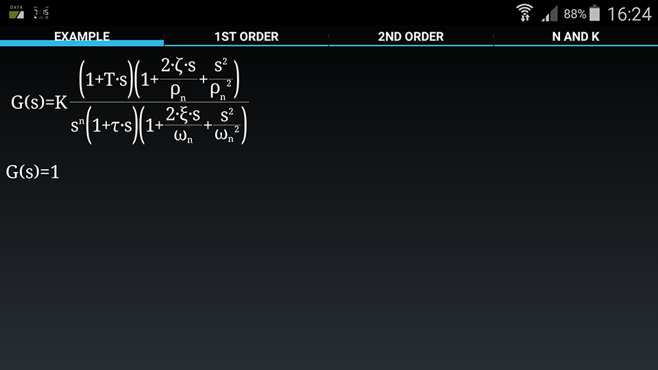
The leftmost tab shows an example of the Bode form, which can be used as a reference to edit the transfer function.

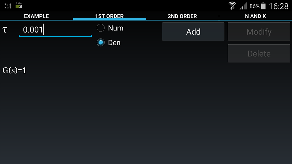
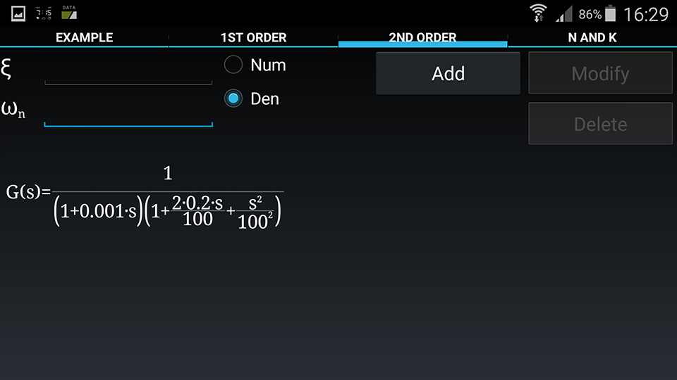
Using the second tab: we can edit the binomial factors. In this example we have just one of these factors in the denominator: insert 0.001 as the value of $\tau$ in the textbox and choose the denominator in the radio buttons.

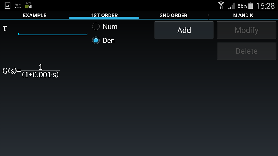
Now you can press the “Add” button, to modify the transfer function. If everything went right, you should have achieved the following result. To select a factor which has to be modified or deleted: just click on the desired factor in the formula below.

Repeat the same process in the “2nd order tab”: insert the value of $\xi$ =0.2 and $\omega_n$ =100 as shown in the following picture.

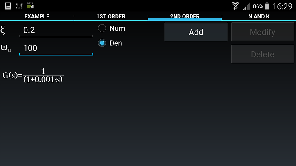
Now press the “Add” button.

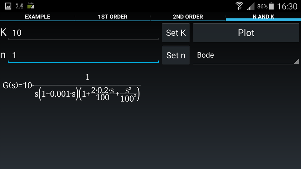
In the last tab, we will edit the values of K=10 and n=1. Insert the values in the proper textboxes and press the buttons “Set K” and “Set n”. To insert poles in the origin you can set the exponent n. Setting n to negative values inserts the desired number of zeroes in the origin.

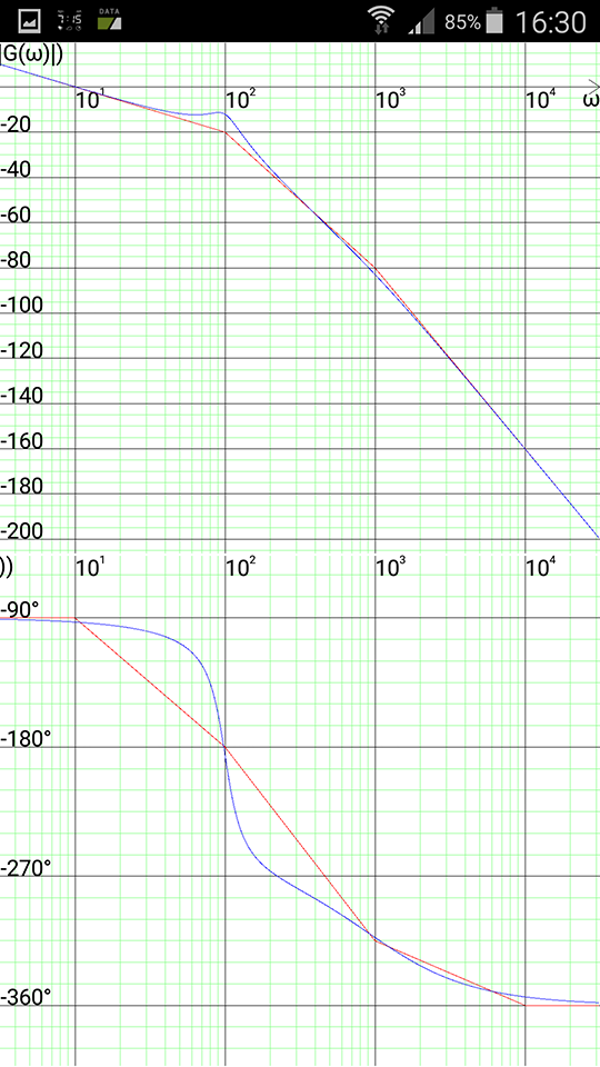
It’s finally time to see our Bode plot: just press the “plot” button. The bode plot shows an upper part which is the representation of the gain, and a lower part, which represents the phase. Both asymptotic (red line) and real (blue line) representations are shown. Each one of the plots can be zoomed or panned just touching the screen. The vertical and horizontal axes can be zoomed independently.

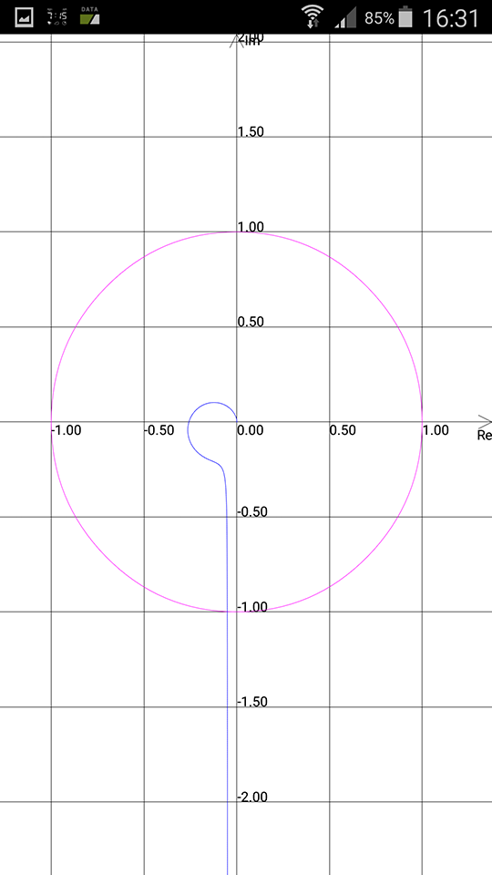
Androbode can also show Nyquist plots: click on the multiple choice box just under the “Plot” button and select “Nyquist”. Click the “Plot” button again.

In the control theory section, several examples have been made available, about the calculation of the parameters in the transfer function.